Marek Hilton

Gnuplot is a fast and flexible plotting tool that produces high quality no nonsense plots. I highly recommend trying it out, particularly if you find yourself automating large amounts of graph plotting and animations. Even for one-off plots for presentation or publication it can quickly produce smart yet informative graphics. For the many things it can do I suggest looking gnuplotting.org, a blog filled with useful plot ideas and gnuplot tutorials.

This said, gnuplot is a somewhat anachronistic tool. The scripting language sometimes lacks consistency. The manuals, though extensive, are difficult to search and are better suited to surfing. Even for a seasoned user of gnuplot, managing and modifying a collection of gnuplot scripts can be a challenge. The language is terse, sometimes irregular, and can often warrant some peculiar, though powerful, hacks to generate more advanced plots or to preprocess data.

In this article I wanted to explain how I’ve been using another vintage command line tool, m4, to alleviate some of these shortcomings. Many of the things I do with m4 macros would probably be better off as feature requests or code contributions to gnuplot. Not to mention, you can only go so far before macros introduce more headaches than they solve. That said, for those in a hurry, they are a quick and dirty way to add more functionality.

The m4 macro preprocessor

The m4 macro preprocessor is a tool from the early days of Unix that still sees use to this day. For example, the GNU autoconf tool makes heavy use of m4. I won’t give a full exposition of its syntax and capabilities here. The GNU documentation is a thorough enough reference. Macros are written in much the same as a function calls in C-like languages:

foo(bar, baz)

-> hello bar, hello baz

and definitions of these macros are themselves are made with the define macro:

define(foo, `hello $1, hello $2')dnl

Only the macro, and not the line, is replaced by its expansion and so macros can be placed anywhere in the text and still be expanded. This is, for example, in contrast to roff macros. This is also why the define macro is usually followed by m4’s comment delimiter (dnl for delete to newline). Without it, after expansion of define() the new line will be left over resulting in a blank line in the file.

Calling gnuplot scripts via m4

Text files that contain m4 macros need to be passed through the preprocessor to expand the macros. For gnuplot scripts with embedded m4 macros, which I usually suffix with .plt.m4, this can be easily done through process substitution in the call to gnuplot:

gnuplot -c <(m4 -Iinclude script.plt.m4)

Note that this requires a shell capable of process substitution such as bash. Alternatively scripts can be supplied through standard input.

m4 -Iinclude script.plt.m4 | gnuplot

I find it’s best to include scripts with m4 macros rather than using gnuplot’s native include mechanism. This means included files can also be preprocessed. Use m4’s -I argument to specify the directories where included files can be found.

In both cases there is a downside in that the input to gnuplot is not seekable so the script cannot invoke itself (fork itself). The solution to this is a simple shell script but is probably the subject of a future post.

Automatic style management

Style management in gnuplot is quite powerful but the labelling of styles is numeric and opaque to the reader. When managing styles across multiple plots I often find myself forgetting which numbers refer to which styles. I also end up overwriting existing styles with later definitions.

You can get around this limitation by defining macros for style management. Below is a macro that takes a name, a style number, and a style definition and creates a new style and an alias for it.

define(def_ls,
`set style line $2 $3
ls_$1 = $2')dnl

Admittedly, this is only really a shorthand for a marginal amount of boilerplate. We can make this macro more terse and useful by removing the style number argument and adding automatic numbering of styles. This can be achieved by using m4’s arithmetic operators.

define(`_style_counter', `9')dnl
define(`style_counter', `define(`_style_counter', incr(_style_counter))dnl
_style_counter')dnl

define(def_ls,
`set style line style_counter $2
ls_$1 = _style_counter')dnl

First we define a macro that acts like a global variable, _style_counter, and a macro, style_counter, that increments the _style_counter and expands to the new value. ¹ On each call to the def_ls macro, we use the counter to generate a new style number. We start the style number at 9 so that the first style number generated is 10 and we retain gnuplot’s default styles.

Putting this together we can use this macro to quickly set line styles with comprehensible names.

def_ls(dashed_red, lc "red" dt 2)
def_ls(thick_dotted_blue, lc "blue" dt (10,5) lw 2)

plot sin(x) ls ls_thick_dotted_blue, cos(x) ls ls_dashed_red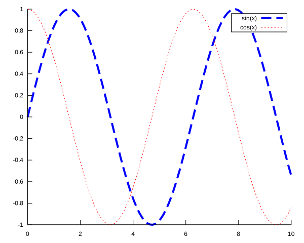

Managing plot resolution and scale

One of the common problems found in articles and papers produced by academics, typically using tools like LaTeX, is that the figures are often scaled wrong (particularly text) and at low resolution. There are usually two fixes to this. Firstly, you can use scalable vector graphics like SVG but this is not always possible either because the data is not suitable or because the word processing software you’re using can’t handle it. Another issue is that they are displayed differently in different contexts, precisely due to the fact that they are scalable. The alternative is to produce a raster graphic like a PNG at the appropriate DPI (dots per inch). This usually manifests as people generating PNGs at a DPI that far exceeds the quality of their final document and then scaling down the PNG to fit the document.

Size and scale

In Gnuplot, it is possible to produce documents at the correct size, resolution, and font size right off the bat. You produce the plot at the on-page intended size and include them in text documents without resizing. Let’s see how to do this with the pngcairo terminal and some m4 macros. First we can define macros to specify width and height.

define(m4_default,`ifelse($1,`',$2,$1)')dnl

define(`m4_pngcairo_set_width',
`define(`m4_pngcairo_width',$1)dnl
define(`m4_pngcairo_width_unit',`m4_default($2,`cm')')dnl)
')dnl

m4_pngcairo_set_width(12,cm)dnl

define(`m4_pngcairo_set_height',
`define(`m4_pngcairo_height',$1)dnl
define(`m4_pngcairo_height_unit',`m4_default($2,`cm')')dnl)
')dnl

m4_pngcairo_set_height(9,cm)dnl

Each macro sets a global variable for width/height and takes two arguments. The first argument is the value and the second argument is and optional unit of measurement. If no unit is specified then it defaults to cm. After each macro definition we also specify a default width and height.

We also specify a macro to configure the DPI of our plot. Unfortunately, I have found that the pngcairo terminal, although plotting in the correct DPI, does not set the dpi in the resulting PNG. To overcome this we also define a macro that sends the output through a imagemagick to fix this.

define(`m4_pngcairo_set_dpi',
`define(`m4_pngcairo_dpi',$1)dnl')dnl

m4_pngcairo_set_dpi(600)dnl

define(`m4_pngcairo_set_output',`set output "| magick - -density m4_pngcairo_dpi $1"')dnl

Finally, we can define a macro that sets up our terminal correctly to produce files of the given size and resolution. Note, in our macro we use a Gnuplot variable to calculate the correct scale from the dpi global variable.

define(m4_pngcairo,
`scale = m4_pngcairo_dpi/96.0
set term pngcairo\
         size (m4_pngcairo_width*scale)m4_pngcairo_width_unit,(m4_pngcairo_height*scale)m4_pngcairo_height_unit\
         fontscale scale\
         pointscale scale\
         linewidth scale\
         transparent rounded
')dnl

To produce a plot with size 9cm x 3cm and a DPI of 128, all we need to do is:

m4_pngcairo_set_width(9,cm)
m4_pngcairo_set_height(3,cm)
m4_pngcairo_set_dpi(128)
m4_pngcairo()
m4_pngcairo_set_output("my_plot.png")

plot cos(x), sin(x)

When including the resulting plot into, for example, a LaTeX file, we simply include the plot at its native size in the document with \includegraphics{my_plot}, perhaps within a center environment. The resulting image will be 9cm x 3cm and as long as the width of the text is 9cm or greater, there will be no overflow.

Font

For some reason, on my machine, the pngcairo terminal scales the font incorrectly by 1.25. This problem is quickly solved with a simple macro that handles picking the font size for you.

define(m4_font,`sprintf("$1,%0.02f",m4_default($2,10)*0.75)dnl')dnl

define(m4_pngcairo_default_font,`m4_font(Nimbus Roman, 10)dnl')dnl

Now when defining the font of a title we can specify the font in the native point size of the document. This means that we can use exactly the same font family and size in both our text document and our plot.²

set title "My awesome plot" font m4_font(Latin Modern Math,14)

Miscellaneous uses

There are lots of little uses for macros in gnuplot so here are a few:

• The dnl comment delimiter is very useful for commenting out curves in a plot command. Since the preprocessor will remove the entire line, line continuations (i.e. the \ at the end of each line) are preserved. This does not happen with Gnuplot comments using a #. This also allows m4 comments to be placed after line continuations unlike Gnuplot comments.
• Including a Gnuplot script in another using gnuplot’s include is to some extent path dependent. You can change the loadpath in order to load files from a specific directory but perhaps easier is to just use m4’s include mechanism. The loadpath can then be used solely for acquiring the relevant data files.